Components tour

OmegaGW composes three swappable parts:

• perturbations — the curvature spectrum \(\mathcal{P}_\zeta(k)\);
• kernel — the transfer function for the source era;
• integrator — the numerical quadrature over the internal momenta \((s,t)\).

This page walks through the options for each, plus the shared inference interface.

import jax
jax.config.update("jax_enable_x64", True)
import jax.numpy as jnp

from sigway.spectrum import OmegaGW
from sigway.kernels import RadiationKernel, InstantEMDKernel
from sigway.perturbations import (
    AnalyticPerturbations, SingleFieldPerturbations,
)
from sigway.ms_solver import SingleFieldSolver
from sigway.binned_pzeta import Binned_P_zeta

1. Perturbations — the spectrum \(\mathcal{P}_\zeta(k)\)

A ScalarPerturbations object evaluates \(\mathcal{P}_\zeta(k,\theta)\) and carries its parameter names. There are three ways to get one.

(a) Analytic — a closed form

AnalyticPerturbations(func, names) wraps any callable func(k, *params). If a parameter sits inside an integration limit (e.g. a sharp cutoff \(k_{\max}\)), flag it with nonsmooth_params so the Jacobian differentiates it by finite differences:

src = AnalyticPerturbations(
    pzeta_flat_cutoff, ("As", "kmax"), nonsmooth_params=("kmax",)
)

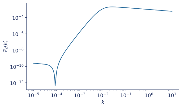
(b) Single-field inflation — solve Mukhanov–Sasaki

SingleFieldPerturbations wraps a SingleFieldSolver, which integrates the background and the mode equations for a potential \(V(\phi)\) and returns \(\mathcal{P}_\zeta\). The potential below has a quasi-inflection point (ultra-slow-roll) tuned to stay CMB-consistent while enhancing small-scale power.

def usr_potential(phi, a, lam, v, nfac):
    b = (1 + nfac) * (1 - a**2/3 + a**2/3 * (9/(2*a**2) - 1)**(2/3))
    x = phi / v
    return lam * v**4/12 * x**2 * (6 - 4*a*x + 3*x**2) / (1 + b*x**2)**2

solver = SingleFieldSolver(
    usr_potential, phi0=3.0, pi0=0.0, N_CMB_to_end=58.0,
    k=jnp.geomspace(1e-5, 10.0, 200),
)
usr_pert = SingleFieldPerturbations(solver, ("a", "lam", "v", "nfac"))
usr_params = (0.71224, 1.47312e-06, 0.19689, 1.86902e-05)

k = jnp.geomspace(1e-5, 10.0, 200)
pzeta = usr_pert(k, *usr_params)        # P_zeta array from the solver

(c) Binned — model-independent

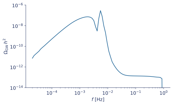
Binned_P_zeta represents \(\mathcal{P}_\zeta\) as free log-amplitudes in \(k\)-bins — fit or forecast the spectrum without committing to a template. It is itself a full model (precomputed coefficients, no \((s,t)\) integral) but exposes the same interface.

binned = Binned_P_zeta("binned", "Binned", nbins=100)
binned.parameter_names              # ('A_0', 'A_1', ..., 'A_99')

amps = [-4.0] * len(binned.parameter_names)   # log10 bin amplitudes
amps[50] = 0.0                                # excite one bin
f_b = jnp.geomspace(2e-5, 1.0, 80)
omega_binned = binned(f_b, *amps)

2. Kernels — the source era

Swapping the kernel changes the cosmology:

• RadiationKernel — radiation domination; \(k\)-independent (the simple example).
• InstantEMDKernel — an early matter-dominated era ending in a sudden transition to radiation; \(k\)-dependent and contributing one parameter, the transition time etaR.

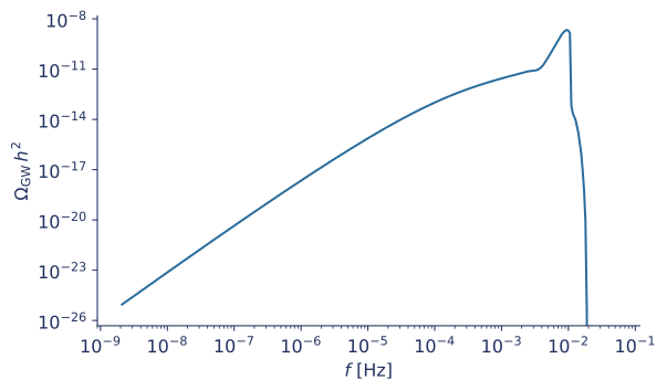
Here the source is flat with a sharp cutoff at kmax:

def pzeta_flat_cutoff(k, As, kmax):
    return jnp.heaviside(kmax - k, 1.0) * As

def t_emd(k, As, kmax, etaR):           # range must reach the cutoff
    return jnp.geomspace(1e-10 * jnp.ones_like(k), 2 * kmax / k, 100)

emd_source = AnalyticPerturbations(
    pzeta_flat_cutoff, ("As", "kmax"), nonsmooth_params=("kmax",)
)
emd_model = OmegaGW(
    emd_source, InstantEMDKernel(),
    s=jnp.linspace(0.0, 1.0, 100), t=t_emd,
)
emd_model.parameter_names               # ('As', 'kmax', 'etaR')

f_emd = jnp.geomspace(2.1e-9, 5e-2, 350)
omega_emd = emd_model(f_emd, As=2.1e-9, kmax=0.06, etaR=2000.0)

3. Integrators — the \((s,t)\) quadrature

The integrator owns the numerical method. The default is SimpsonIntegrator(s, t) — fixed-grid Simpson quadrature over the two internal momenta; passing s= and t= to OmegaGW builds one for you. Two practical points:

• Grid spacing matters more than point count. The integrand has a sharp feature near \(t\lesssim1\) and a long tail above; linear below 1, geometric above captures both, while pure log-spacing at the same count can leave the integral ~10 % high.
• The grid can depend on \(k\) and the parameters — pass a callable t(k, *theta) (like t_emd above) so the range adapts to the source:

def t_adaptive(k, logAs, logDelta, logks):
    ks = 10.0**logks
    upper = jnp.exp(4 * 10.0**logDelta) * (2 * ks / k)
    lo = jnp.linspace(1e-5, 0.999, 200) * jnp.ones_like(k)
    hi = jnp.geomspace(jnp.ones_like(k), upper, 600)
    return jnp.concatenate([lo, hi], axis=0)

To use a different scheme entirely, subclass Integrator and pass it as integrator=.

4. The shared inference interface

Every model — analytic, single-field or binned — exposes one ordered parameter vector and an autodiff Jacobian \(\partial\Omega_{\mathrm{GW}}/\partial\theta\), the building block of a Fisher forecast (forward-mode autodiff, with finite differences for nonsmooth_params).

f = jnp.geomspace(1e-5, 1e-1, 200)
theta = [-2.5, -0.30103, -2.0]
jac = model.jacobian(f, theta)      # shape (len(f), n_params)

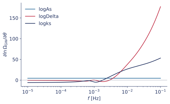
The curves are \(\partial \ln \Omega_{\mathrm{GW}}/\partial\theta\) — the dimensionless response of the spectrum to each parameter.

---

Download this example as a notebook — the runnable version, including the plotting code.