Simple example

The smallest end-to-end calculation: take a primordial curvature power spectrum \(\mathcal{P}_\zeta(k)\), pick a kernel (the transfer function for the source era), and get the induced GW spectrum \(\Omega_{\mathrm{GW}}(f)\) — three objects composed into one OmegaGW model.

import jax
jax.config.update("jax_enable_x64", True)   # SIGW integrals need float64
import jax.numpy as jnp

from sigway.spectrum import OmegaGW
from sigway.kernels import RadiationKernel
from sigway.perturbations import AnalyticPerturbations

1. A primordial power spectrum

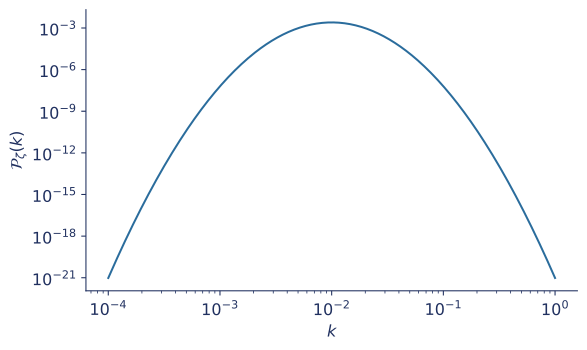
We use a log-normal peak — a bump of curvature power on a characteristic scale \(k_\star\), with three knobs:

param	meaning
logAs	\(\log_{10}\) of the integrated amplitude \(A_s\)
logDelta	\(\log_{10}\) of the dimensionless width \(\Delta\)
logks	\(\log_{10}\) of the peak wavenumber \(k_\star\)

\[\mathcal{P}_\zeta(k) = \frac{A_s}{\sqrt{2\pi}\,\Delta}\, \exp\!\left[-\frac{\ln^2(k/k_\star)}{2\Delta^2}\right].\]

def pzeta_lognormal(k, logAs, logDelta, logks):
    As = 10.0**logAs
    Delta = 10.0**logDelta
    ks = 10.0**logks
    norm = As / (jnp.sqrt(2 * jnp.pi) * Delta)
    return norm * jnp.exp(-0.5 / Delta**2 * jnp.log(k / ks)**2)

params = (-2.5, -0.30103, -2.0)   # logAs, logDelta, logks (peak at k=0.01)
k = jnp.geomspace(1e-4, 1e0, 400)
pzeta = pzeta_lognormal(k, *params)

2. Build the model

Wrap the callable in AnalyticPerturbations (with its parameter names), choose the radiation-domination kernel, and pass two integration grids: s \(\in[0,1]\) (the angular internal momentum) and t (the radial one — linear below 1, geometric above it captures both the resonance and the tail).

s = jnp.linspace(0.0, 1.0, 10)
t = jnp.concatenate([
    jnp.linspace(1e-5, 0.999, 200),
    jnp.geomspace(1.0, 1e3, 800),
])

perts = AnalyticPerturbations(
    pzeta_lognormal, ("logAs", "logDelta", "logks")
)
model = OmegaGW(perts, RadiationKernel(), s=s, t=t)

model.parameter_names        # ('logAs', 'logDelta', 'logks')

3. Evaluate

The model is callable — give it the frequencies and parameters (positional in parameter_names order, or by keyword). The first call JIT-compiles; later calls are fast.

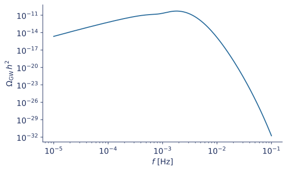
f = jnp.geomspace(1e-5, 1e-1, 200)
omega = model(f, *params)    # == model(f, logAs=-2.5, logDelta=-0.30103, logks=-2.0)

What the knobs do

• logAs scales the whole signal: \(\Omega_{\mathrm{GW}}\propto A_s^2\) (two powers of \(\mathcal{P}_\zeta\) enter the source).
• logks slides the GW bump in frequency (the peak tracks \(k_\star\)).
• logDelta sets how broad the bump is.

---

Download this example as a notebook — the runnable version, including the plotting code. Next: the components tour.